Summary
The two-sample independent t-test is used to determine whether the means of two independent groups differ significantly.
It is applied when data are continuous, observations are independent, and the goal is to compare group averages.
Key assumptions include normality, independence of observations, and homogeneity of variances.
Variance equality is tested using Bartlett’s, Levene’s, or F-test.
If variances are equal, the pooled t-test is used; otherwise, Welch’s t-test is preferred.
In the given examples, equal variances led to no significant mean difference, while unequal variance cases require Welch’s approach.
1. Introduction
A two-sample independent t-test is a statistical method used to determine if there is a significant difference between the means of two independent groups.
This test is particularly useful in comparing the average performance, outcomes or measurements of two distinct groups to understand if they significantly differ from each other, beyond what might be expected by random chance.
2. When to use two sample T-Test
The two-sample t-test, also known as the independent samples t-test, is used to compare the means of two independent groups to determine if there is a statistically significant difference between them.
3. Assumption of two sample independent T-Test
For the two-sample independent t-test to be valid, certain assumptions must be met:
- Independence of observation: The observations in each group must be independent of each other. This means that the measurement of one participant should not influence or be related to the measurement of another participant within the same group or across groups.
- Normality: The data in each group should be approximately normally distributed. This assumption is particularly important for small sample sizes (n < 30).
- Homogeneity of variance: The variances of the two groups should be equal. This assumption is known as homoscedasticity. If the variances are not equal, a modified version of the t-test, known as Two sample independent t-test with unequal variance (Welch's t-test), should be used. The Levene's test or F-test can be used to check for equality of variances.
- Scale of measurement: The variables should be continuous and have meaningful numerical values with equal intervals between them.
4. Step to check assumptions:
- Normality: Use graphical methods such as histograms or Q-Q plots to visually inspect the distribution of the data. Conduct normality tests like the Shapiro-Wilk test or Kolmogorov-Smirnov test.
- Homogeneity of variance: TPerform Levene's test, the F-test and Bartlett’s test to check if the variances of the two groups are significantly different.
1. Two sample independent t-test with equal variance
The two-sample t-test with equal variance assesses whether there is a significant difference between the means of two independent groups.
This statistical test assumes homogeneity of variances and normal distribution within each group, making it suitable for comparing the means of two normally distributed populations.
Checking homogeneity of variance by Bartlett’s test:
Bartlett's test evaluates the homogeneity of variances across multiple samples. By calculating a test statistic from the sample variances, it determines if there are significant differences. A p-value below a chosen significance level (e.g., 0.05) indicates unequal variances, while a higher p-value suggests equal variances.
Formula of Bartlett’s Test
The test statistic \( T \) for Bartlett’s test is given by:
\[
T =
\left( \frac{N - k}{C} \right) \ln \left( s_p^2 \right)
-
\sum_{i=1}^{k}
\left( \frac{n_i - 1}{C} \right)
\ln \left( s_i^2 \right)
\]
Where,
\[
\begin{aligned}
k & : \text{Number of groups} \\
n_i & : \text{Number of observations in the } i^{\text{th}} \text{ group} \\
N & : \text{Total number of observations across all groups} \\
s_i^2 & : \text{Variance of the } i^{\text{th}} \text{ group} \\
s_p^2 & : \text{Pooled variance}
\end{aligned}
\]
\[
C =
1 +
\frac{1}{3(k - 1)}
\left(
\sum_{i=1}^{k} (\frac{1}{n_i - 1})
-
\frac{1}{N - k}
\right)
\]
\[
s_p^2 =
\frac{1}{N - k}
\sum_{i=1}^{k}
(n_i - 1)s_i^2
\]
The test statistic \( T \) follows a chi-squared distribution with
\( k - 1 \) degrees of freedom.
Example of Bartlett’s test:
A study is conducted to compare the effectiveness of two different teaching methods (Method A and Method B) on student test scores. The experiment involves two groups of students, with 10 students in each group.
The test scores of the students are recorded after they have been taught using their respective methods.
- Method A: 60, 65, 70, 75, 80, 85, 90, 95, 100, 105
- Method B: 55, 60, 65, 70, 75, 80, 85, 90, 95, 100
Solution:
Hypothesis:
- Null hypothesis (H0): The variances of the test scores for both methods are equal.
- Alternative hypothesis (H1): The variances of the test scores for both methods are not equal.
Bartlett's Test:
-
Calculate the variance for each group:
-
For Method A:
\[
\text{Mean}=
\frac{60 + 65 + 70 + \cdots + 105}{10}
= 82.5
\]
\[
\text{Variance}=
\frac{(60 - 82.5)^2 + (65 - 82.5)^2 + \cdots + (105 - 82.5)^2}{10 - 1}
= 229.165
\]
-
For Method B:
\[
\text{Mean}=
\frac{55 + 60 + \cdots + 100}{10}
= 77.5
\]
\[
\text{Variance}=
\frac{(55 - 77.5)^2 + (60 - 77.5)^2 + \cdots + (100 \bar{ + } 77.5)^2}{10 - 1}
= 229.165
\]
-
Calculate pooled variance:
\[
s_p^2 =
\frac{1}{10 + 10 - 2}
\left[
(10 - 1)* 275 + (10 - 1)* 275
\right]
= 229.165
\]
-
Calculate the correction factor:
\[
C =
1 +
\frac{1}{3(2 - 1)}
\left(
\frac{1}{10 - 1}
+
\frac{1}{10 - 1}
-
\frac{1}{10 + 10 - 2}
\right)
= 1.0555
\]
-
Calculate the test statistic \( T \):
\[
T =
\left(
\frac{10 + 10 - 2}{1.0555}
\right)
\ln(229.165)
-
2
\left(
\frac{10 - 1}{1.0555}
\right)
\ln(229.165)
= 0
\]
Determine the p-value:
The test statistic T follows a chi-squared distribution with k – 1 = 2 - 1 = 1 degree of freedom.
In this case, T = 0, corresponding to a very high p-value (1).
Thus, we do not reject the null hypothesis of equal variances.
Conclusion:
Based on Bartlett's test,
there is no significant evidence to suggest that the variances of test scores differ between Method A and Method B.
To perform a two-sample independent t-test with equal variances based on the provided example, we'll use the test to compare the means of the test scores for Method A and Method B.
Hypothesis:
- Null hypothesis (H0): The means of the test scores for Method A and Method B are equal.
- Alternative hypothesis (H1): The means of the test scores for Method A and Method B are not equal.
-
Calculate the Mean and Variance for each group:
-
For Method A:
\[
\bar{X}_1 =
\frac{60 + 65 + 70 + \cdots + 105}{10}
= 82.5
\]
\[
s_1^2 =
\frac{(60 - 82.5)^2 + (65 - 82.5)^2 + \cdots + (105 - 82.5)^2}{10 - 1}
= 229.165
\]
-
For Method B:
\[
\bar{X}_2 =
\frac{55 + 60 + \cdots + 100}{10}
= 77.5
\]
\[
s_2^2 =
\frac{(55 - 77.5)^2 + (60 - 77.5)^2 + \cdots + (100 \bar{ + } 77.5)^2}{10 - 1}
= 229.165
\]
-
Calculate pooled variance:
\[
s_p^2 =
\frac{1}{n_1 + n_2 - 2}
\left[
(n_1 - 1)s_1^2 + (n_2 - 1) s_2^2
\right]
\]
\[
s_p^2 =
\frac{1}{10 + 10 - 2}
\left[
(10 - 1)* 275 + (10 - 1)* 275
\right]
= 229.165
\]
-
Calculate the standard error:
\[
SE =
\sqrt{
s_p^2
\left(
\frac{1}{n_1} + \frac{1}{n_2}
\right)
}
\]
\[
SE =
\sqrt{
229.167
\left(
\frac{1}{10} + \frac{1}{10}
\right)
}
= 6.77
\]
-
Calculate the t-statistic:
\[
t =
\frac{\bar{X}_1 - \bar{X}_2}{SE}
\]
\[
t =
\frac{82.5 - 77.5}{6.77}
= 0.7385
\]
-
Determine the degrees of freedom:
\[
df = n_1 + n_2 - 2 = 10 + 10 - 2 = 18
\]
Find the critical value:
For a two tailed test with = 0.05 and df = 18, the critical value is approximately 2.101.
Compare the t-statistic and critical value:
Calculated t (0.7385) is less than critical value of t (2.101), so we fail to reject null hypothesis.
Conclusion: There is not enough evidence to reject the null hypothesis.
This suggests that there is no significant difference in the mean test scores between Method A and Method B.
2. Two sample independent t-test with unequal variance:
The two-sample t-test with unequal variances, also known as Welch's t-test, compares the means of two independent groups when their variances differ. It's robust when the assumption of equal variances is violated.
Welch's t-test adjusts the degrees of freedom and provides a more reliable comparison under heterogeneous variances.
Example of Two sample independent t-test with unequal variance:
A new variety of cotton was evolved by a breeder. In order to compare its yielding ability with that of a ruling variety, an experiment was conducted in CRD. The kapas yield (kg/plot) was observed.
The summary of the results are given below. Test whether the new variety of cotton gives higher yield than the ruling variety.
| New variety |
Ruling variety |
| \[ n_1 = 9 \] |
\[ n_2 = 11 \] |
| \[ \bar{X}_1 = 28.2 \] |
\[ \bar{X}_2 = 25.9 \] |
| \[ s_1^2 = 5.4430 \] |
\[ s_2^2 = 1.2822 \] |
Check homogeneity of variance:
-
Calculate pooled variance:
\[
s_p^2 =
\frac{1}{9 + 11 - 2}
\left[
(9 - 1)\times 5.4430 + (11 - 1)\times 1.2822
\right]
= 3.1314
\]
-
Calculate the correction factor:
\[
C =
1 +
\frac{1}{3(2 - 1)}
\left(
\frac{1}{9 - 1}
+
\frac{1}{11 - 1}
-
\frac{1}{9 + 11 - 2}
\right)
= 1.0933
\]
-
Calculate the test statistic \( T \):
\[
T =
\left(
\frac{9 + 11 - 2}{1.0933}
\right)\ln(3.1314)
-
\left(
\frac{9 - 1}{1.0933}
\right)\ln(5.4430)
-
\left(
\frac{11 - 1}{1.0933}
\right)\ln(1.2822)
= 4.116
\]
-
Determine the p-value:
The test statistic \( T \) follows a chi-squared distribution
with \( k - 1 = 2 - 1 = 1 \) degree of freedom.
In this case, \( T = 4.116 \), corresponding to a very low
p-value (0.042). Thus, we reject the null hypothesis of
equal variances.
Calculate the standard error:
\[
SE =
\sqrt{
\frac{s_1^2}{n_1}
+
\frac{s_2^2}{n_2}
}
\]
\[
SE =
\sqrt{
\frac{5.4430}{9}
+
\frac{1.2822}{11}
}
= 0.8494
\]
Calculate the t-statistic:
\[
t =
\frac{\bar{X}_1 - \bar{X}_2}{SE}
\]
\[
t =
\frac{28.2 - 25.9}{0.8494}
= 2.708
\]
This statistic follows neither the t-distribution nor the normal distribution.
It follows what is known as the Behrens – Fisher d - distribution.
The Behrens – Fisher test is laborious one. An alternative simple method has been
suggested by Cochran and Cox. In this method, the critical value of \( t \)
is altered as:
\[
t_w =
\frac{
t_1\left(\dfrac{s_1^2}{n_1}\right)
+
t_2\left(\dfrac{s_2^2}{n_2}\right)
}{
\dfrac{s_1^2}{n_1}
+
\dfrac{s_2^2}{n_2}
}
\]
Where \( t_1 = 2.306 \) is the critical value for \( n_1 - 1 \) df
at the specificlevel of significance, (0.05), t2 (2.228) is the critical value
for \( n_2 - 1 \) df at the same level of significance.
\[
t_w =
\frac{
(2.306)(0.6048)
+
(2.228)(0.1166)
}{
(0.6048)
+
(0.1166)
}
= 2.293
\]
Conclusion:
Since \( t > t_w \), we reject the null hypothesis that the two cotton varieties
give similar yield. Since \( \bar{X}_1 > \bar{X}_2 \), we conclude that the new
variety of cotton gives significantly higher yield of kapas than the ruling
variety.
Same Problem analysis in Agri Analyze:
Problem analysis in Agri Analyze:
The best part of performing analysis with AgriAnalyze is that auto interpretation along with assumption testing.
Step 1:Go to the website https://www.agrianalyze.com/TwoSamplePairedTTest.aspx
(For first time users free registration is mandatory)
Step 2:Prepare data in csv file as shown below:
| Method_A |
Method_B |
| 60 |
55 |
| 65 |
60 |
| 70 |
65 |
| 75 |
70 |
| 80 |
75 |
| 85 |
80 |
| 90 |
85 |
| 95 |
90 |
| 100 |
95 |
| 105 |
100 |
Step 3: Link Here to download sample file Sample File Download
Step 4: Upload data, select conditions for variance of samples, add level of significance, add variable name and category type.
Step 5: Click submit, pay a nominal fee, and download the output report with detailed interpretation.
Output Report:
Link of the output report
Video Tutorial:
Link of the Youtube Tutorial
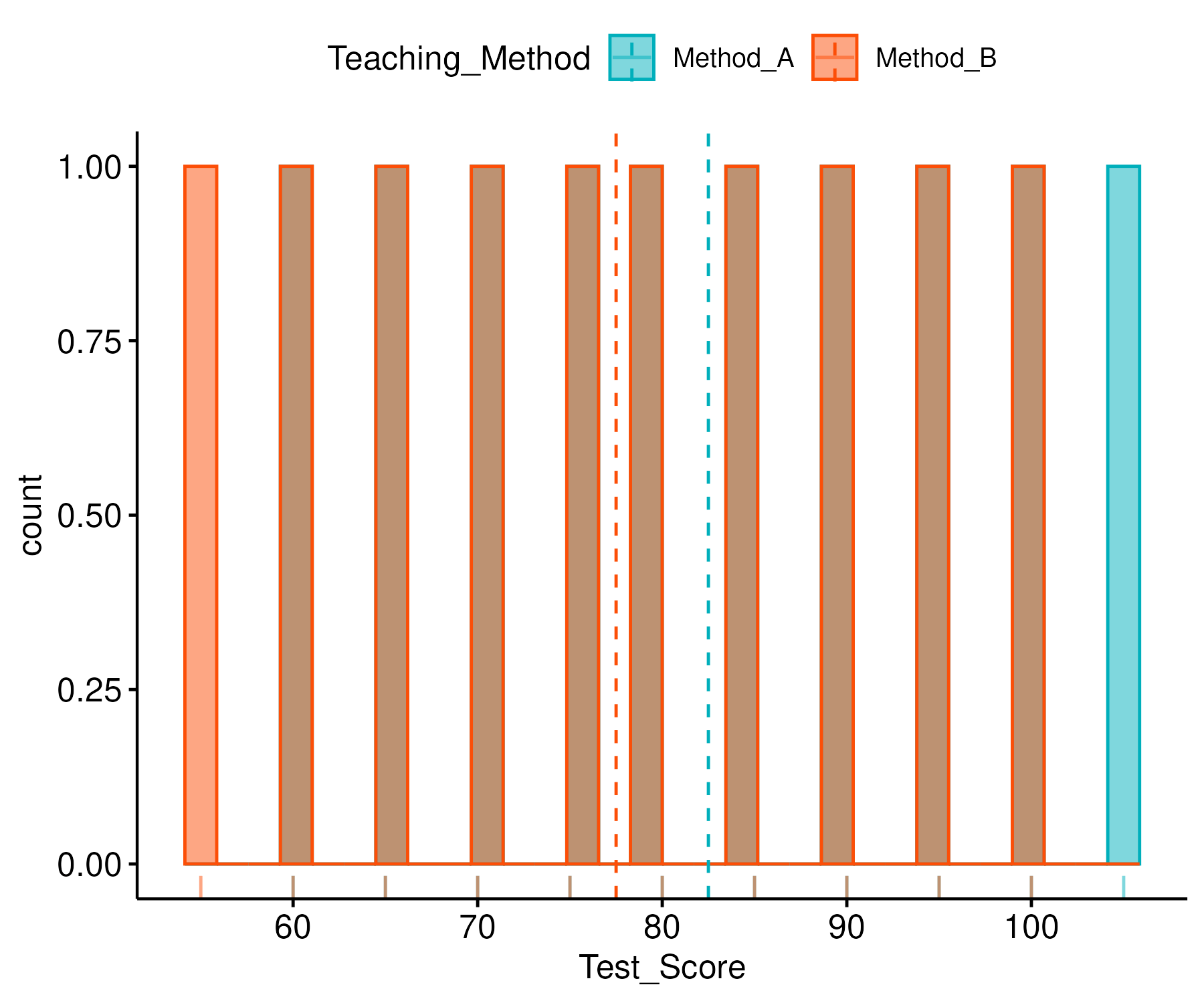
Descriptive Statistics of Data
| Statistics |
Method_A |
Method_B |
| Mean |
\( 82.500 \) |
\( 77.500 \) |
| Median |
\( 82.500 \) |
\( 77.500 \) |
| Variance |
\( 229.167 \) |
\( 229.167 \) |
| Standard Deviation |
\( 15.138 \) |
\( 15.138 \) |
| Coefficient of Variation |
\( 18.349 \) |
\( 19.533 \) |
| Skewness |
\( 0.000 \) |
\( 0.000 \) |
| Kurtosis |
\( -1.562 \) |
\( -1.562 \) |
Diagram :
Histogram Plot:
Box Plot:

Shapiro Wilk test for checking normality of the Method_A
Null hypothesis (Ho):
The Test_Score data of Method_A sample is normally distributed.
Alternative Hypothesis (Ha):
The Test_Score data of Method_A sample is not normally distributed.
Results:
Shapiro-Wilk test statistic: 0.97016 and P-value: 0.89237
Interpretation:
The p value 0.8924 is greater than alpha value ( 0.05 ).
The results are non-significant and we accept the null hypothesis. The data is normally distributed.
Shapiro Wilk test for checking normality of the Method_B
Null hypothesis (Ho):
The Test_Score data of Method_B sample is normally distributed.
Alternative Hypothesis (Ha):
The Test_Score data of Method_B sample is not normally distributed.
Results:
Shapiro-Wilk test statistic: 0.97016 and P-value: 0.89237
Interpretation:
The p value 0.8924 is greater than alpha value ( 0.05 ).
The results are non-significant and we accept the null hypothesis. The data is normally distributed.
Bartlett's test for testing homogeneity of variances for both the samples
Null hypothesis (Ho): The variances of both the samples are homogenous
Results:
Bartlett's test statistic 0 p value: 1
Interpretation:
As the p value 1 is greater than aplha 0.05 .
The result is non-significant and null hypothesis is accepted. The variances of both the samples are homogenous.
Results of the two sample independent t-test
Ho:μ 1 = μ 2 (The population Test_Score mean of both the samples are equal)
Ha:μ 1 ≠ μ 2 (The population Test_Score mean of both the samples are not equal)
| Particulars |
Value |
| Particulars |
Value |
| Mean of Method\_A |
\( 82.5 \) |
| Mean of Method\_B |
\( 77.5 \) |
| Assumption of Variance |
Variances are homogeneous |
| Degrees of Freedom |
\( 18 \) |
| \( t \) value |
\( 0.7385 \) |
| Standard Error |
\( 6.77 \) |
| \( p \) value |
\( 0.4697 \) |
| Lower limit of Confidence Interval |
\( -9.2233 \) |
| Upper limit of Confidence Interval |
\( 19.2233 \) |
Interpretation:
The p value 0.469 was greater than alpha ( 0.05 ).
The results were non-significant and we accept the null hypothesis.
The population Test_Score mean of both the sample are equal.
Reference
Agri Analyze website for analysis,
Rangaswamy R. (1995). A text book of Agricultural Statistics. New Age International.
The blog is written by:
Darshan Kothiya, PhD Scholar, Department of Agricultural Statistics, BACA, AAU, Anand