Summary
The paired t-test is a statistical method used to compare the means of two related groups, such as measurements taken before and after a treatment. This blog explains when and why the paired t-test is used, along with its key assumptions and differences from the independent t-test. A solved example using milk production data from cows illustrates the step-by-step analysis. The blog also demonstrates how the same test can be easily performed using Agri Analyze with automatic interpretation and reporting.
1. Introduction
A paired t-test compares the means of two related groups to determine if there is a statistically significant difference between them.
This test is used when the same subjects are measured twice, such as before and after a treatment.
By analyzing the differences between paired observations, the paired t-test accounts for variability within subjects,
making it a powerful tool for detecting changes or effects in experiments and repeated-measures studies.
2. When to Use Paired t-Test
A paired t-test is used to compare the means of two related groups to determine if there is a statistically significant difference.
This test is applicable when the same subjects are measured twice or when pairs of related subjects are matched.
- The same subjects are measured twice (e.g., before and after treatment).
- Pairs of related subjects are matched based on specific criteria.
- The objective is to detect significant changes within subjects by analyzing paired differences.
3. Assumptions of Paired t-Test
- Paired Observations: Data consists of related pairs (e.g., before and after measurements).
- Continuous Data: Differences are measured on interval or ratio scale.
- Normality: Differences between paired observations are approximately normally distributed.
- Independence: Each pair is independent of other pairs.
- Scale of Measurement: Data should be at least interval level.
4. Difference Between Paired t-Test and Independent t-Test
The paired t-test compares the means of two related groups by focusing on within-subject differences.
In contrast, the two-sample independent t-test compares the means of two unrelated groups.
The paired t-test controls for within-subject variability, whereas the independent t-test evaluates differences between separate groups.
5. Solved Example
The following table shows the milk production (in liters) of 12 cows during morning and evening milking.
Test whether milk production is the same for both times.
| Cow |
Morning (Xi) |
Evening (Yi) |
Cow |
Morning (Xi) |
Evening (Yi) |
| 1 |
4.5 |
4.0 |
7 |
5.0 |
4.5 |
| 2 |
5.6 |
4.5 |
8 |
7.5 |
7.5 |
| 3 |
7.5 |
7.5 |
9 |
10.5 |
10.0 |
| 4 |
8.0 |
7.6 |
10 |
7.0 |
7.0 |
| 5 |
8.0 |
5.5 |
11 |
10.0 |
9.5 |
| 6 |
8.5 |
8.5 |
12 |
8.5 |
8.5 |
Procedure for Paired t-Test
Step 1: Hypothesis
Null Hypothesis (H0):
The mean difference between the paired observations is zero.
H0: μd = 0
Step 2: Level of Significance
Fix the level of significance. Usually, 5% (0.05) and 1% (0.01) levels of significance are used.
Step 3: Calculation of Required Statistics
(i) Calculate the difference for each pair:
di = Xi − Yi
| Cow |
Morning (Xi) |
Evening (Yi) |
di = Xi − Yi |
di2 |
| 1 |
4.5 |
4.0 |
0.5 |
0.25 |
| 2 |
5.6 |
4.5 |
1.1 |
1.21 |
| 3 |
7.5 |
7.5 |
0.0 |
0.00 |
| 4 |
8.0 |
7.6 |
0.4 |
0.16 |
| 5 |
8.0 |
5.5 |
2.5 |
6.25 |
| 6 |
8.5 |
8.5 |
0.0 |
0.00 |
| 7 |
5.0 |
4.5 |
0.5 |
0.25 |
| 8 |
7.5 |
7.5 |
0.0 |
0.00 |
| 9 |
10.5 |
10.0 |
0.5 |
0.25 |
| 10 |
7.0 |
7.0 |
0.0 |
0.00 |
| 11 |
10.0 |
9.5 |
0.5 |
0.25 |
| 12 |
8.5 |
8.5 |
0.0 |
0.00 |
| Total |
6.0 |
8.62 |
(ii) Mean difference:
\[
\bar{d} = \frac{\sum d_i}{n} = \frac{6}{12} = 0.5
\]
(iii) Sample variance:
\[
S^2 = \frac{\sum (d_i - \bar{d})^2}{n - 1} = 0.5109
\]
(iv) Standard error of mean difference:
\[
SE(\bar{d}) =
\sqrt{\frac{S^2}{n}} =
\sqrt{\frac{\sum (d_i - \bar{d})^2}{n(n-1)}} =
\sqrt{\frac{0.5109}{12}} = 0.2063
\]
Step 4: Test Statistic
\[
t = \frac{\lvert \bar{d} - \mu_d \rvert }{SE(\bar{d})}
= \frac{0.5}{0.2063}
= 2.42
\]
Step 5: Conclusion
If calculated t (2.42) > table t (0.05,n-1) (2.20),
observed difference is significant at 5% level of significance
and the null hypothesis is rejected at 5% level of significance.
Rejection of null hypothesis means the milk production of both the time is not same.
6. Same Problem Analysis Using Agri Analyze
The best part of performing analysis with Agri Analyze is that auto interpretation along with assumption testing.
Step 1: Open https://www.agrianalyze.com/PairedTTest
(First-time users must complete free registration)
Step 2: Prepare the dataset in CSV format as shown above.
Milk Production Data (Morning vs Evening)
| Morning |
Evening |
| 4.5 |
4.0 |
| 5.6 |
4.5 |
| 7.5 |
7.5 |
| 8.0 |
7.6 |
| 8.0 |
5.5 |
| 8.5 |
8.5 |
| 5.0 |
4.5 |
| 7.5 |
7.5 |
| 10.5 |
10.0 |
| 7.0 |
7.0 |
| 10.0 |
9.5 |
| 8.5 |
8.5 |
Step 3: Upload the data and enter the following details:
- Add level of Significance: we have kept 0.05 i.e. 5%;
- Add variable name : Milk production in Liter
- Category Type: As we are comparing milk production in Morning and Evening we have wrote "Time of Milking"
Step 4: Click submit, pay a nominal fee, and download the output report with detailed interpretation.
Output Report:
Link of the output report
Video Tutorial:
Link of the Youtube Tutorial
Output Interpretation :
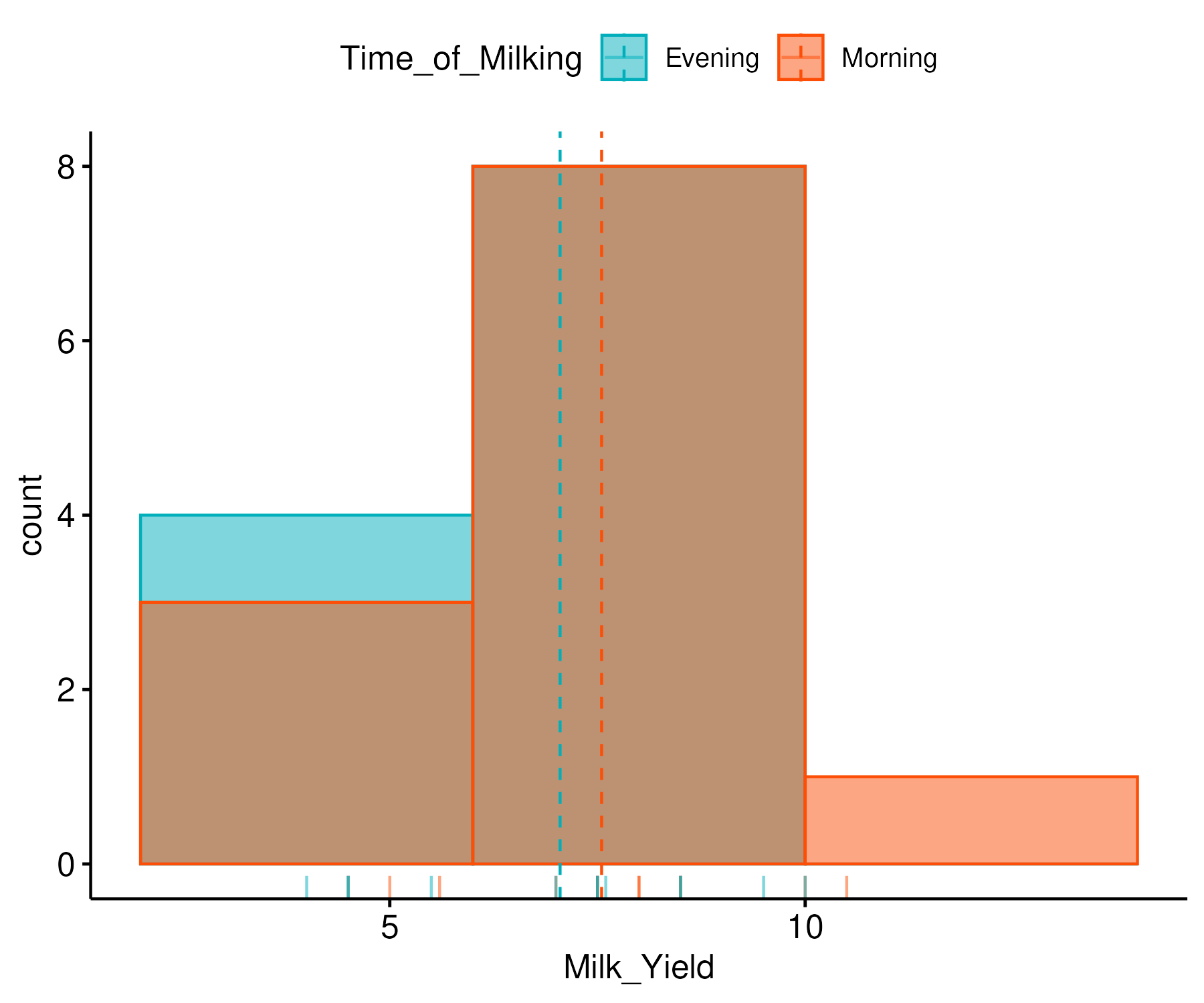
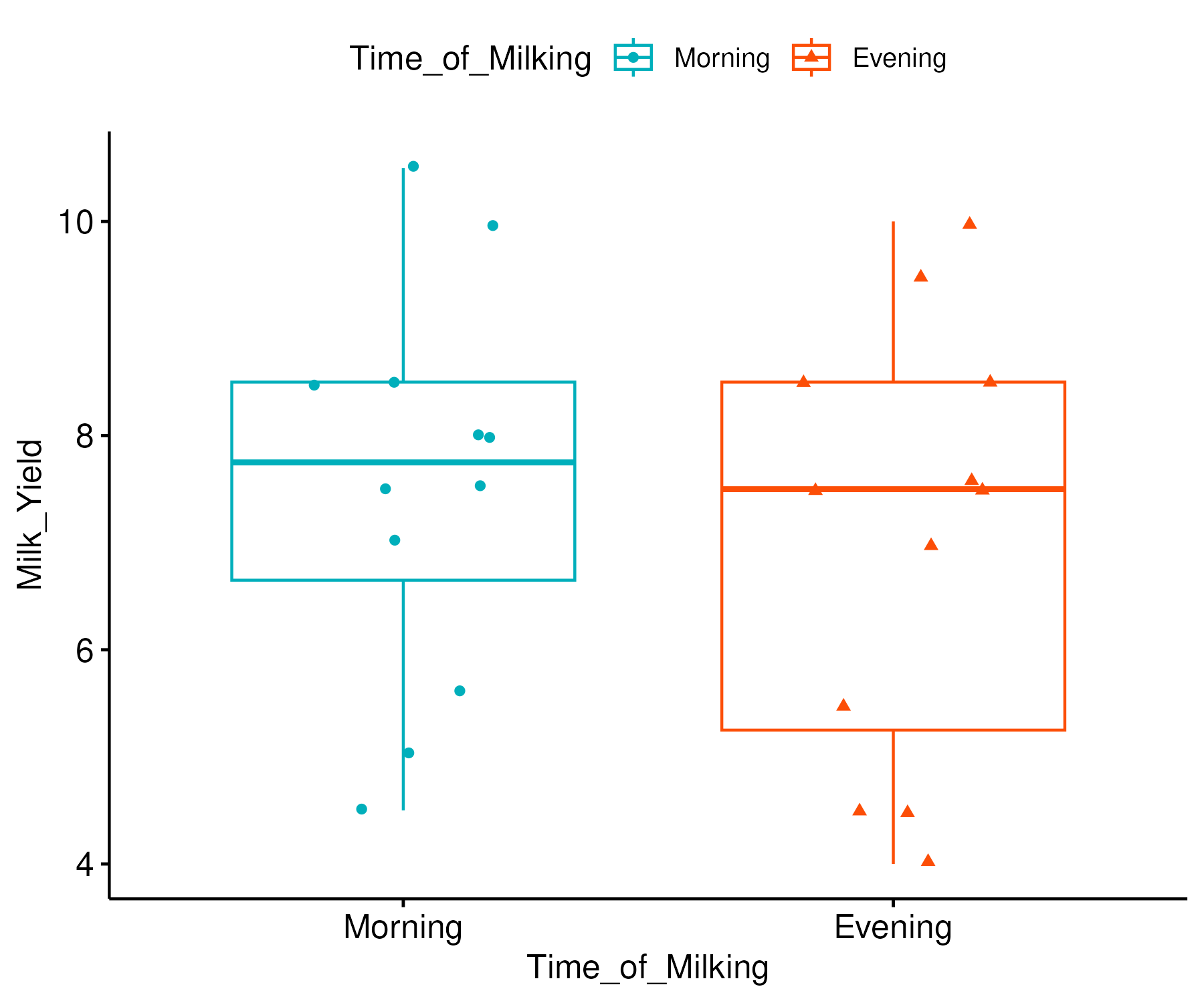
Descriptive Statistic of Data
| Statistics |
Morning |
Evening |
| Mean |
7.550 |
7.050 |
| Median |
7.750 |
7.500 |
| Variance |
3.348 |
4.030 |
| Standard Deviation |
1.830 |
2.007 |
| Coefficient of variation |
24.238 |
28.468 |
| Skewness |
-0.140 |
-0.190 |
| Kurtosis |
-1.091 |
-1.473 |
Diagram :
Histogram Plot:
Box Plot:
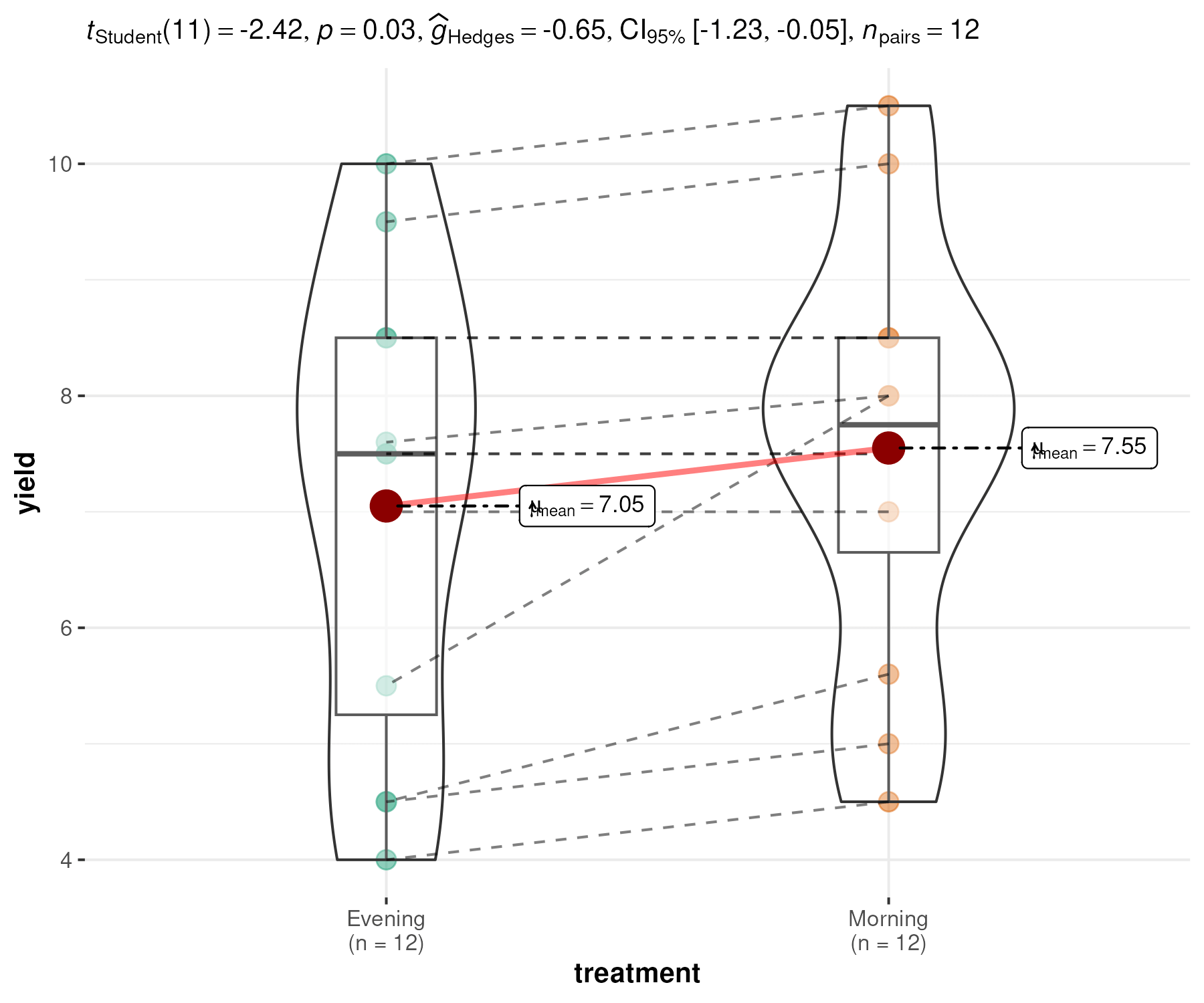
Additional Plot:
Shapiro Wilk test for checking normality of the difference between both samples
Null hypothesis (Ho):
The difference of both the category is normally distributed
Alternative Hypothesis (Ha):
The difference of both the category is not normally distributed
Results:
Shapiro-Wilk test statistic: 0.69784 and P-value: 8e-04
Interpretation:
The p value 8e-04 is less than alpha value (0.05).
The results are significant and we fail to accept the null hypothesis.
The data is not normally distributed.
Results of the paired t test
Ho: (Average Difference between two samples) d = 0
Ha: (Average Difference between two samples) d ≠ 0
| Particulars |
Value |
| Mean diff. between sample (By user) |
0.0000 |
| Degrees of Freedom |
11.0000 |
| t value |
2.4232 |
| Standard Error |
0.2063 |
| P value |
0.0338 |
| Lower limit of Conf. interval |
0.0459 |
| Upper limit of Conf. interval |
0.9541 |
| Mean Difference |
0.5000 |
Interpretation:
The p value 0.0338 was less than alpha (0.05).
The results were significant and we fail to accept the null hypothesis.
The mean difference between two sample for the variable
Milk_Yield is not equal to 0.
Reference
Gupta, S. C., & Kapoor, V. K. (2020). Fundamentals of Mathematical Statistics. Sultan Chand & Sons.
The blog is written by:
Darshan Kothiya, PhD Scholar, Department of Agricultural Statistics, BACA, AAU, Anand