Summary
The one-sample t-test is used to determine whether a sample mean differs significantly from a known or hypothesized population mean.
This blog explains when and why the test is used, along with its key assumptions and formula.
A solved IQ-based example demonstrates hypothesis testing, p-value interpretation, and confidence interval estimation.
The analysis shows how non-significant results lead to accepting the null hypothesis. Finally, the blog illustrates how the same test can be easily performed using the Agri Analyze tool with automatic calculation and interpretation.
1.Introduction
The one-sample t-test is a statistical method used to determine if the mean of a single sample is significantly different from a known or hypothesized population mean.
It is widely used in various fields to test hypotheses about population means when the population standard deviation is unknown and the sample size is relatively small.
2.Definition
You should use a one-sample t-test when you want to compare the mean of a sample to a specific value, typically a known population mean or a hypothesized value.
This test is particularly useful when:
- You have a single sample of data.
- The population standard deviation is unknown.
- The sample size is small (usually n < 30)
3.Assumptions of a One-Sample T-Test
For the one-sample t-test to be valid, certain assumptions must be met:
- Independence:The observations in the sample must be independent of each other.
- Normality:The data should be approximately normally distributed. This assumption is particularly important for small sample sizes.
- Scale of Measurement: The data should be continuous and measured at an interval or ratio scale.
4.How is One-Sample T-Test Different from Two-Sample and Paired T-Tests?
- One-Sample T-Test: Compares the mean of a single sample to a known or hypothesized population mean.
- Two-Sample T-Test: Compares the means of two independent samples to determine if they are significantly different from each other.
- Paired T-Test:Compares the means of two related groups (e.g., measurements before and after an intervention) to determine if there is a significant difference.
5. Formula
The formula for the one-sample t-test is:
$$
t = \frac{\bar{x} - \mu}{\dfrac{s}{\sqrt{n}}}
$$
Where:
- \(\bar{x}\) is the sample mean
- \(\mu\) is the population mean (hypothesized mean)
- \(s\) is the sample standard deviation
- \(n\) is the number of observations
6. How to interpret the results?
Case1:If the p value is greater than alpha value the results are non significant and the null hypothesis is accepted.
Case2: If the p value is less than or equal to alpha value the results are significant and the null hypothesis is rejected.
7. Solved example
A random sample of 10 boys had the following IQ's: 70, 120, 110, 101, 88, 83, 95, 98, 107, 100. Do these data support the assumption of the population mean IQ of 100 ?
Find a reasonable range in which most of the mean IQ values of the population of boys lie. (Use alpha 0.05)
Step 1:Formation of Null Hypothesis
\( \text{Null Hypothesis } H_0 : \mu = 100 \)
\( \text{Alternative Hypothesis } H_a : \mu \ne 100 \)
Step 2:Computation of mean, sample standard deviation and t test
Sample Mean = (70+120+...+107+100)/10 = 972/10 = 97.20
\[
s^2 =
\frac{\sum (70 - 97.2)^2 + (120 - 97.2)^2 + \cdots + (100 - 97.2)^2}{10 - 1}
= 203.73
\]
\[
|t| =
\frac{|97.2 - 100|}{\sqrt{\dfrac{203.73}{10}}}
= 0.62
\]
Step 3: Compute p-value
The p value can be obtained in the excel by using the formula =TDIST(t cal, degrees of freedom, tail of the test). For our case =TDIST(0.62, 9, 2). The p value is 0.5506.
Step 4: Conclusion
The p value 0.5506 is greater than alpha value 0.05, results are non significant and the null hypothesis is accepted.
This means that at 5% level of significance data is consistent with the assumption of mean IQ of 100 for the population of boys.
Step 5: Confidence Interval Computation
\[
\text{Confidence interval limit 95% } =
\text{Sample Mean} \pm t(\text{df}, 5\%) \times \sqrt{\frac{s^2}{n}}
\]
\[
= 97.2 \pm 2.26 \times \sqrt{\frac{203.73}{10}}
= 97.2 \pm 10.21
\]
\[
\text{Lower Limit} = 86.99
\qquad
\text{Upper Limit} = 107.41
\]
The t value at 9 degrees of freedom and 5% level of significance was =TINV(0.05,9) = 2.2621.
Same problem analysis in Agri Analyze:
The best part of performing analysis with Agri Analyze is that auto interpretation along with assumption testing.
Step 1:Open link https://agrianalyze.com/OneSampleTTest.aspx (For first time users free registration is mandatory)
Step 2:Prepare data file and save in a csv format
| Observation |
IQ |
| 1 |
70 |
| 2 |
120 |
| 3 |
110 |
| 4 |
101 |
| 5 |
88 |
| 6 |
83 |
| 7 |
95 |
| 8 |
98 |
| 9 |
107 |
| 10 |
100 |
Step 3: Link Here to download sample file Sample File Download
Step 4:
- Upload data,
- Select Alpha level of significance (for 5% write 0.05) ,
- Mean Value = 50
Step 5: Click submit, pay a nominal fee, and download the output report with detailed interpretation.
Output Report:
Link of the output report
Video Tutorial:
Link of the Youtube Tutorial
Descriptive Statistics of Data
| Statistic |
Y_{1900} |
| Mean |
97.200 |
| Median |
99.000 |
| Variance |
203.733 |
| Standard Deviation |
14.274 |
| Coefficient of Variation |
14.685 |
| Skewness |
-0.303 |
| Kurtosis |
-0.827 |
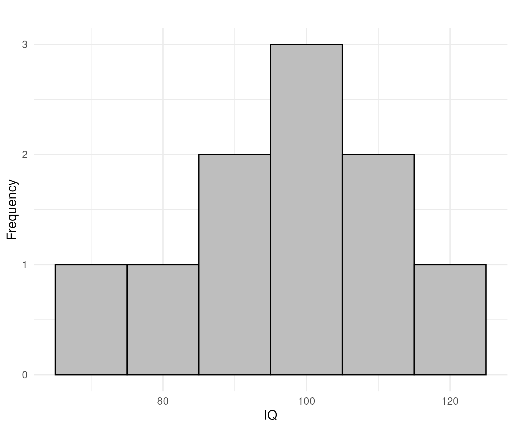
Diagram :
Histogram Plot:
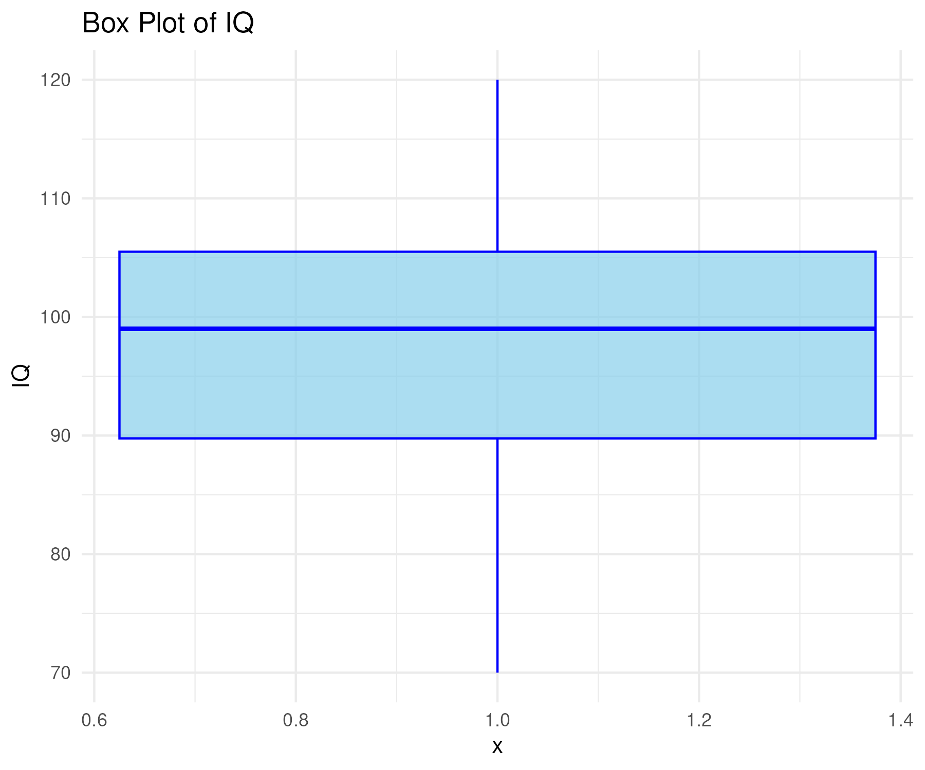
Box Plot:
Shapiro Wilk test for checking Normality of Data
Null hypothesis (Ho):
The data is normally distributed
Null hypothesis (Ha):
The data is not normally distributed
Results:
Shapiro-Wilk test statistic: 0.98311 and P-value: 0.97964
Interpretation:
The p value 0.9796 is greater than alpha value ( 0.05 ).
The results are non-significant and we accept the null hypothesis.
The data is normally distributed
Results of the t test
Ho: (Population Mean) μ = 50
Ho: (Population Mean) μ ≠ 50
| Particulars |
Value |
| Hypothetical Mean |
50.0000 |
| Degrees of Freedom |
9.0000 |
| t Value |
10.4571 |
| Standard Error |
4.5137 |
| P Value |
0.0000 |
| Lower Limit of Confidence Interval |
86.9893 |
| Upper Limit of Confidence Interval |
107.4107 |
| Sample Mean |
97.2000 |
Interpretation:
The p value 2.463, was less than alpha ( 0.05 ).
The results were significant and we fail to accept the null hypothesis The mean of the IQ is not equal to 50 .
Reference
Gupta, S. C., & Kapoor, V. K. (2020). Fundamentals of mathematical statistics. Sultan Chand & Sons.