Summary
The F-test is a statistical method used to compare the variances of two populations or samples to determine whether they are significantly different.
Commonly applied in regression analysis, ANOVA, and model fitting, the test assumes independent samples, normality, and homogeneity of variances.
By calculating the ratio of sample variances and comparing it with critical values from the F-distribution, a decision is made to accept or reject the null hypothesis of equal variances.
The blog explains the theory, assumptions, hypothesis formulation, and step-by-step procedure of the F-test, followed by a real-life example using life expectancy data from Brazil.
It also demonstrates how the F-test can be easily performed using the Agri Analyze platform with automated results and interpretation.
1.Introduction
The F-test is a statistical method used to compare the variances of two samples or the ratio of variances across multiple samples.
It assesses whether the data follow an F-distribution under the null hypothesis, assuming standard conditions for the error term (ε).
The test statistic, denoted as F, is commonly used to compare fitted models to determine which best represents the underlying population.
F-tests are frequently employed in models fitted using least squares.
The test is named after Ronald Fisher, who introduced the concept as the "variance ratio" in the 1920s, with George W. Snedecor later naming the test in Fisher’s honor.
2.Definition
An F-test uses the F-statistic to evaluate whether the variances of two samples (or populations) are equal.
The test assumes that the population follows an F-distribution and that the samples are independent.
If the F-test yields statistically significant results, the null hypothesis of equal variances is rejected; otherwise, it is not.
3.Use of F-Test in Statistics
The F-test is a statistical tool used to compare variances and determine if there are significant differences between two populations or samples.
It is commonly applied in regression analysis, statistical inference, model fitting, and analysis of variance (ANOVA) to identify the best-fitting statistical model or assess differences across groups.
- Regression analysis
- Statistical inference
- Model fitting
- Analysis of variance (ANOVA)
Assumptions
- Independence:The observations within each group must be independent, meaning there should be no relationship between observations across samples.
- Normality: Data in each group should follow a normal distribution. For large sample sizes, this assumption can be relaxed based on the Central Limit Theorem.
- Homogeneity of variances:The variances across groups being compared should be approximately equal.
Important Notes on the F-Test
- The F-test is used to assess whether the variances of two populations are equal by comparing them using an F distribution.
- The F-test statistic is calculated as
\( F = \frac{s_1^2}{s_2^2} \),
where \( s_1^2 \) and \( s_2^2 \) are the sample variances.
- The null hypothesis is evaluated using a critical value, which determines whether to reject the hypothesis.
- A common application of the F-test is the one-way ANOVA, which assesses variability between group means and within group observations.
Selection Criteria for s12 and s22 in an F-Test
For a right-tailed or two-tailed F-test, the variance with the greater value is placed in the numerator,
making the sample corresponding to s12 the first sample. The smaller variance
(s22) is used as the denominator for the second sample.
For a left-tailed test, the smaller variance is placed in the numerator (sample 1), while the larger
variance is placed in the denominator (sample 2).
Hypotheses
Left-Tailed Test
- Null Hypothesis (H0): σ12 = σ22
- Alternative Hypothesis (H1): σ12 < σ22
- Decision Criteria: Reject H0 if the F-statistic < F-critical value
Right-Tailed Test
- Null Hypothesis (H0): σ12 = σ22
- Alternative Hypothesis (H1): σ12 > σ22
- Decision Criteria: Reject H0 if the F-statistic > F-critical value
Two-Tailed Test
- Null Hypothesis (H0): σ12 = σ22
- Alternative Hypothesis (H1): σ12 ≠ σ22
Procedure for Conducting an F-Test
1. Define Hypotheses
Null Hypothesis (H0): The variances of the groups are equal.
Alternative Hypothesis (H1): The variances of the groups are not equal.
2. Collect Data
Gather sample data from the groups being compared.
3. Calculate Sample Variances
For each group, compute the sample variance (s2) using the formula:
$$
s^2 = \frac{\sum_{i=1}^{n}(x_i - \bar{x})^2}{n-1}
$$
where xi represents the observations, x̄ is the sample mean, and n is the sample size.
4. Calculate F-Statistic
$$
F = \frac{s_1^2}{s_2^2}
$$
where s12 is the larger variance and s22 is the smaller variance.
5. Determine Degrees of Freedom
$$
df_1 = n_1 - 1 \quad \text{(numerator)}
$$
$$
df_2 = n_2 - 1 \quad \text{(denominator)}
$$
6. Find the Critical Value
Using an F-distribution table, locate the critical value for your chosen significance level (e.g., α = 0.05) based on df1 and df2.
7. Make a Decision
- If F > Critical Value, reject the null hypothesis, indicating significant differences in variances.
- If F ≤ Critical Value, fail to reject the null hypothesis, suggesting no significant variance differences.
8. Conclusion
Reject the null hypothesis if F exceeds the critical value, indicating significant variance between groups.
Fail to reject the null hypothesis if F is less than or equal to the critical value, implying insufficient evidence of variance differences.
Example
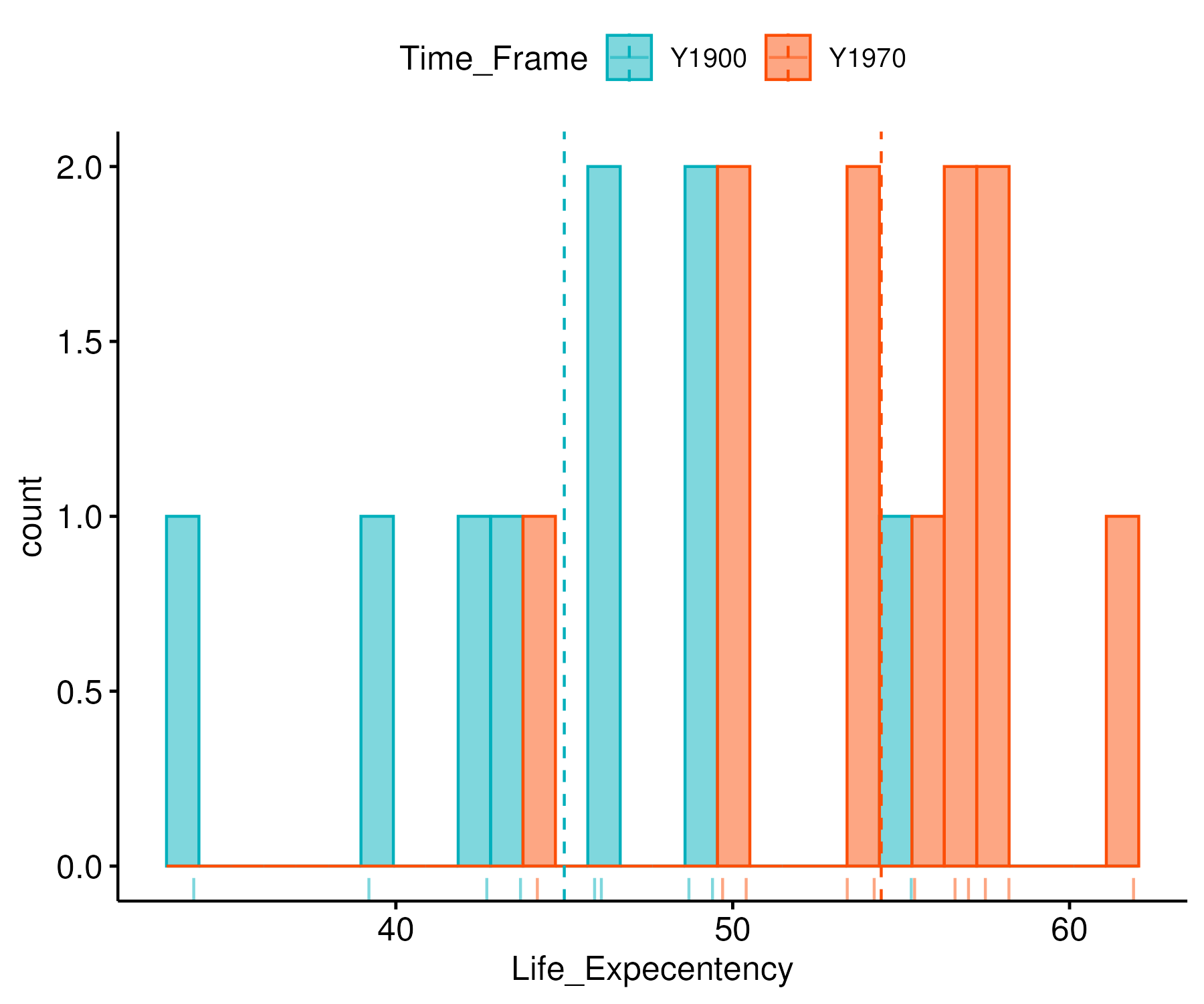
Life expectancy in 9 regions of Brazil in 1900 and 11 regions of Brazil in 1970 is given in the table below:
| Region |
1900 |
1970 |
| 1 |
42.7 |
54.2 |
| 2 |
43.7 |
50.4 |
| 3 |
34.0 |
44.2 |
| 4 |
39.2 |
49.7 |
| 5 |
46.1 |
55.4 |
| 6 |
48.7 |
57.0 |
| 7 |
49.4 |
58.2 |
| 8 |
45.9 |
56.6 |
| 9 |
55.3 |
61.9 |
| 10 |
|
57.5 |
| 11 |
|
53.4 |
We aim to determine whether the variation in life expectancy across regions in 1900 and 1970 is the same.
Assuming the populations in 1900 and 1970 follow normal distributions,
N(μ1, σ12) and
N(μ2, σ22), the hypotheses can be formulated as:
Null Hypothesis (H0):
σ12 = σ22
(the variances are equal)
Alternative Hypothesis (H1):
σ12 ≠ σ22
(the variances are different)
The F-test is applied to evaluate these hypotheses.
1. Calculation of Sample Variances
$$
s_1^2 = \frac{1}{8}
\left(
\sum_{i=1}^{9} x_{1i}^2 - \frac{\left(\sum_{i=1}^{9} x_{1i}\right)^2}{9}
\right)
$$
$$
s_1^2 = \frac{1}{8}\left(18527.78 - \frac{405^2}{9}\right)
= \frac{302.78}{8}
= 37.848
$$
$$
s_2^2 = \frac{1}{10}
\left(
\sum_{j=1}^{11} x_{2j}^2 - \frac{\left(\sum_{j=1}^{11} x_{2j}\right)^2}{11}
\right)
$$
$$
s_2^2 = \frac{1}{10} \left(32799.91 - \frac{598.5^2}{11}\right)
= \frac{236.07}{10}
= 23.607
$$
2. Calculation of the F-Statistic
$$
F = \frac{s_1^2}{s_2^2}
= \frac{37.848}{23.607}
= 1.603
$$
3. Conclusion
The critical values from the F-distribution table at
α = 0.05 for a two-tailed test with degrees of freedom
(8, 10) are
F0.025 = 3.85 and
F0.975 = 0.233.
Since the calculated F-value (1.603) is less than 3.85 and greater than 0.233,
we fail to reject the null hypothesis.
This indicates that there is no significant difference in the variances of life
expectancy between 1900 and 1970 across the regions of Brazil.
F-Test Demonstration in Agri Analyze
Step 1:Go to the website https://www.agrianalyze.com/FTest.aspx
(For first time users free registration is mandatory)
Step 2:Prepare data file and save in a csv format
| Y1900 |
Y1970 |
| 42.7 |
54.2 |
| 43.7 |
50.4 |
| 34 |
44.2 |
| 39.2 |
49.7 |
| 46.1 |
55.4 |
| 48.7 |
57 |
| 49.4 |
58.2 |
| 45.9 |
56.6 |
| 55.3 |
61.9 |
|
57.5 |
|
53.4 |
Step 3: Link Here to download sample file Sample File Download
Step 4:
- Upload data,
- Select level of significance (for 5% write 0.05) ,
- Variable name: Life Expectancy,
- Category Type: Time Frame.
Step 5: Click submit, pay a nominal fee, and download the output report with detailed interpretation.
Output Report:
Link of the output report
Video Tutorial:
Link of the Youtube Tutorial
Descriptive Statistics of Data
| Statistic |
Y_{1900} |
Y_{1970} |
| Mean |
45.0000 |
54.4091 |
| Median |
45.9 |
55.4 |
| Variance |
37.8475 |
23.6069 |
| Standard Deviation |
6.1520 |
4.8587 |
| Coefficient of Variation |
13.6712 |
8.9299 |
| Skewness |
-0.1479 |
-0.5554 |
| Kurtosis |
-0.8573 |
-0.5319 |
Diagram :
Histogram Plot:
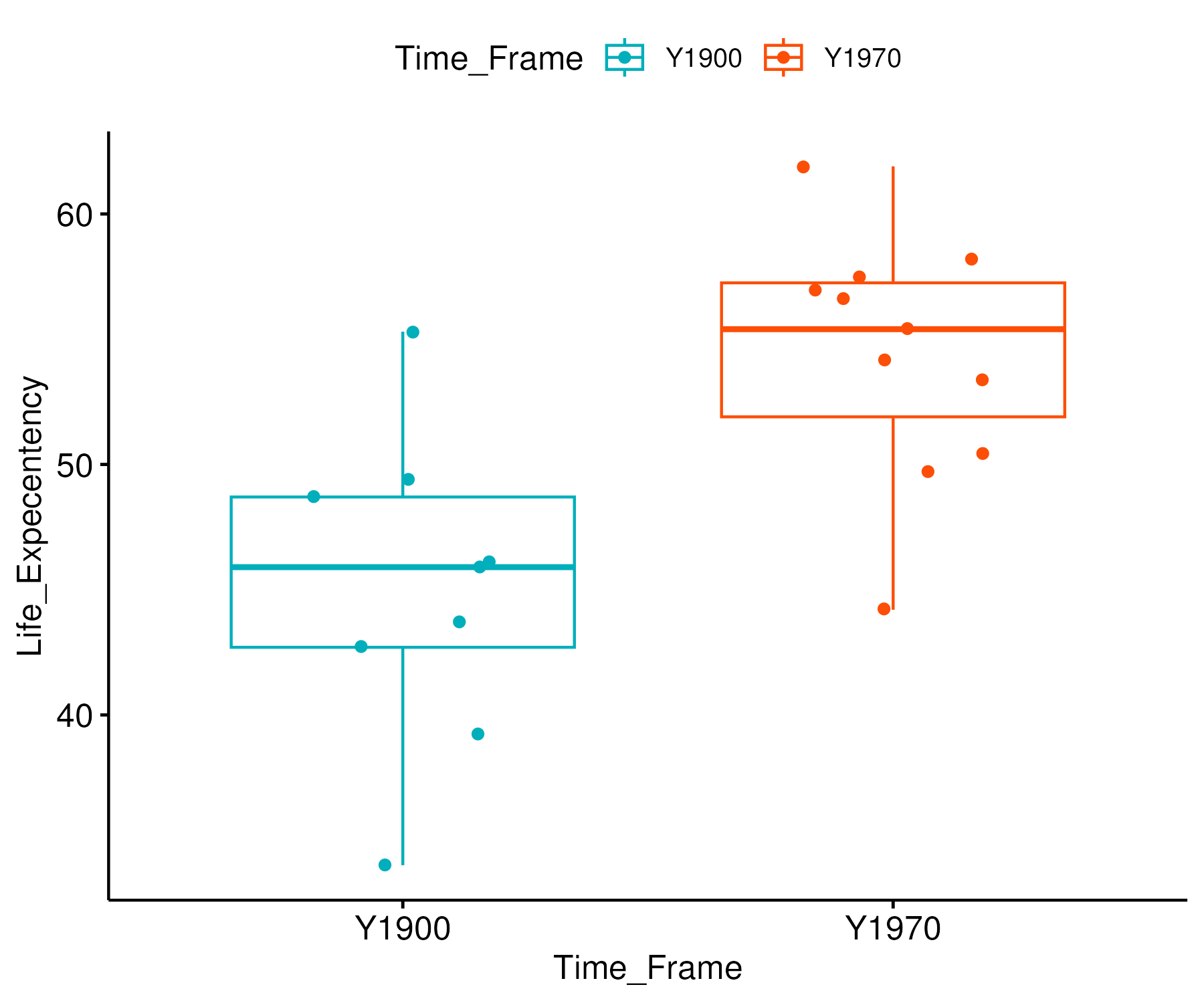
Box Plot:
Shapiro Wilk test for checking normality of the Y1900
Null hypothesis (Ho):
The data of Y1900 sample is normally distributed.
Null hypothesis (Ha):
The data of Y1900 sample is not normally distributed.
Results:
Shapiro-Wilk test statistic: 0.9843 and P-value: 0.9827
Interpretation:
The p value 0.9827 is greater than alpha value ( 0.05 ).
The results are non-significant and we accept the null hypothesis. The data is normally distributed
Shapiro Wilk test for checking normality of the Y1970
Null hypothesis (Ho):
The data of Y1970 sample is normally distributed.
Null Hypothesis (Ha):
The data of Y1970 sample is not normally distributed.
Results:
Wilk test statistic: 0.9554 and P-value: 0.7135
Interpretation:
The p value 0.7135 is greater than alpha value ( 0.05 ).
The results are non-significant and we accept the null hypothesis.
The data is normally distributed.
F Test Results
H0: σ12 = σ22
(The population variance of both the samples are equal)
Ha: σ12 ≠ σ22
(The population variance of both the samples are not equal)
Summary of F Test
| Particulars |
Value |
| Variance 1 |
37.8475 |
| Variance 2 |
23.6069 |
| F-Test Value |
1.6032 |
| P-Value |
0.4762 |
| Degrees of Freedom-1 |
8.0000 |
| Degrees of Freedom-2 |
10.0000 |
| Lower Limit of Confidence Interval |
0.4159 |
| Upper Limit of Confidence Interval |
6.8861 |
Interpretation:
The p-value (0.4762) is greater than alpha (α = 0.05).
The results were non-significant, and we accept the null hypothesis.
The population variances of both samples are equal.
Reference
Agri Analyze website for analysis
The blog is written by:
Uttam Baladaniya, PhD Scholar, Department of Agricultural Statistics, Anand Agricultural University